Modelling infrastructure exposure and risk
This notebook forms the basis of “Hands-On 6” in the CCG course.
It uses the road network and flood dataset extracted in the previous tutorial.
Exposure - overlay sample flood extent with the network and estimate flood depth of exposure
Vulnerability - assume depth-damage curve (fragility curve) for the road and
show how the exposure is translated to damage
create a table with probability, flood depth, length exposed, fragility, cost/km, direct damage
Risk - show a risk calculation on the table and generate the result
Future risk - repeat with climate projections and compare with baseline
By the end of this tutorial you should be able to:
Assess direct damage and indirect disruptions to infrastructure assets
Apply the risk calculation to understand how to generate loss-probability curves
Show how different flood hazards introduce uncertainty in risk estimations
[1]:
# Imports from Python standard library
from pathlib import Path

# Imports from other Python packages
import geopandas as gpd

# numpy is used by pandas and geopandas to store data in efficient arrays
# we use it in this notebook to help with trapezoidal integration
# see https://numpy.org/
import numpy as np
import pandas as pd

# seaborn helps produce more complex plots
# see https://seaborn.pydata.org/
import seaborn as sns

import snail.damages
import snail.intersection
import snail.io
from scipy.integrate import simpson

from pyproj import Geod
Change this to point to your data folder as in the previous tutorial:
[2]:
dir = Path().resolve().parent.parent
data_folder = dir / "ghana_tutorial"
# data_folder = Path("YOUR_PATH/ghana_tutorial")
1. Exposure
List all the hazard files in the flood_layer folder:
[3]:
hazard_paths = sorted(
    (data_folder / "flood_layer" / "gha" / "wri_aqueduct_version_2").glob("wri*.tif")
)

hazard_files = pd.DataFrame({"path": hazard_paths})
hazard_files["key"] = [Path(path).stem for path in hazard_paths]
hazard_files, grids = snail.io.extend_rasters_metadata(hazard_files)

hazard_files.head(5)[["key", "grid_id", "bands"]]
[3]:
| key | grid_id | bands | |
|---|---|---|---|
| 0 | wri_aqueduct-version_2-inuncoast_historical_wt... | 0 | (1,) |
| 1 | wri_aqueduct-version_2-inuncoast_historical_wt... | 0 | (1,) |
| 2 | wri_aqueduct-version_2-inuncoast_historical_wt... | 0 | (1,) |
| 3 | wri_aqueduct-version_2-inuncoast_historical_wt... | 0 | (1,) |
| 4 | wri_aqueduct-version_2-inuncoast_historical_wt... | 0 | (1,) |
[4]:
assert len(grids) == 1
grid = grids[0]
Read in roads again, then do intersections against all hazard scenarios.
[5]:
roads_file = data_folder / "GHA_OSM_roads.gpkg"
roads = gpd.read_file(roads_file, layer="edges")
roads.head(2)
[5]:
| osm_id | road_type | name | id | from_id | to_id | length_m | geometry | |
|---|---|---|---|---|---|---|---|---|
| 0 | 4790594 | tertiary | Airport Road | roade_0 | roadn_0 | roadn_1 | 236.526837 | LINESTRING (-0.17544 5.6055, -0.17418 5.60555,... |
| 1 | 4790599 | tertiary | South Liberation Link | roade_1 | roadn_2 | roadn_10777 | 18.539418 | LINESTRING (-0.17889 5.59979, -0.17872 5.59977) |
[6]:
# split roads along hazard data grid

# TODO top-level "overlay_rasters"
# TODO for vector in vectors / for raster in rasters "overlay_raster"


# push into split_linestrings, flag to disable
prepared = snail.intersection.prepare_linestrings(roads)

flood_intersections = snail.intersection.split_linestrings(prepared, grid)

# push into split_linestrings
flood_intersections = snail.intersection.apply_indices(
    flood_intersections, grid, index_i="i_0", index_j="j_0"
)

flood_intersections = snail.io.associate_raster_files(flood_intersections, hazard_files)

# calculate the length of each stretch of road
# don't include in snail wrapper top-level function
geod = Geod(ellps="WGS84")
flood_intersections["length_m"] = flood_intersections.geometry.apply(
    geod.geometry_length
)
[7]:
# save to file
output_file = (
    data_folder
    / "results"
    / Path(roads_file).name.replace(".gpkg", "_edges___exposure.geoparquet")
)

flood_intersections.to_parquet(output_file)
[8]:
list(flood_intersections.columns)[:21]
[8]:
['osm_id',
 'road_type',
 'name',
 'id',
 'from_id',
 'to_id',
 'length_m',
 'geometry',
 'split',
 'i_0',
 'j_0',
 'wri_aqueduct-version_2-inuncoast_historical_wtsub_2030_rp0001_5-gha',
 'wri_aqueduct-version_2-inuncoast_historical_wtsub_2030_rp0002_0-gha',
 'wri_aqueduct-version_2-inuncoast_historical_wtsub_2030_rp0005_0-gha',
 'wri_aqueduct-version_2-inuncoast_historical_wtsub_2030_rp0010_0-gha',
 'wri_aqueduct-version_2-inuncoast_historical_wtsub_2030_rp0025_0-gha',
 'wri_aqueduct-version_2-inuncoast_historical_wtsub_2030_rp0050_0-gha',
 'wri_aqueduct-version_2-inuncoast_historical_wtsub_2030_rp0100_0-gha',
 'wri_aqueduct-version_2-inuncoast_historical_wtsub_2030_rp0250_0-gha',
 'wri_aqueduct-version_2-inuncoast_historical_wtsub_2030_rp0500_0-gha',
 'wri_aqueduct-version_2-inuncoast_historical_wtsub_2030_rp1000_0-gha']
[9]:
data_cols = [col for col in flood_intersections.columns if "wri" in col]
[10]:
data_cols[:20]
[10]:
['wri_aqueduct-version_2-inuncoast_historical_wtsub_2030_rp0001_5-gha',
 'wri_aqueduct-version_2-inuncoast_historical_wtsub_2030_rp0002_0-gha',
 'wri_aqueduct-version_2-inuncoast_historical_wtsub_2030_rp0005_0-gha',
 'wri_aqueduct-version_2-inuncoast_historical_wtsub_2030_rp0010_0-gha',
 'wri_aqueduct-version_2-inuncoast_historical_wtsub_2030_rp0025_0-gha',
 'wri_aqueduct-version_2-inuncoast_historical_wtsub_2030_rp0050_0-gha',
 'wri_aqueduct-version_2-inuncoast_historical_wtsub_2030_rp0100_0-gha',
 'wri_aqueduct-version_2-inuncoast_historical_wtsub_2030_rp0250_0-gha',
 'wri_aqueduct-version_2-inuncoast_historical_wtsub_2030_rp0500_0-gha',
 'wri_aqueduct-version_2-inuncoast_historical_wtsub_2030_rp1000_0-gha',
 'wri_aqueduct-version_2-inuncoast_historical_wtsub_2050_rp0001_5-gha',
 'wri_aqueduct-version_2-inuncoast_historical_wtsub_2050_rp0002_0-gha',
 'wri_aqueduct-version_2-inuncoast_historical_wtsub_2050_rp0005_0-gha',
 'wri_aqueduct-version_2-inuncoast_historical_wtsub_2050_rp0010_0-gha',
 'wri_aqueduct-version_2-inuncoast_historical_wtsub_2050_rp0025_0-gha',
 'wri_aqueduct-version_2-inuncoast_historical_wtsub_2050_rp0050_0-gha',
 'wri_aqueduct-version_2-inuncoast_historical_wtsub_2050_rp0100_0-gha',
 'wri_aqueduct-version_2-inuncoast_historical_wtsub_2050_rp0250_0-gha',
 'wri_aqueduct-version_2-inuncoast_historical_wtsub_2050_rp0500_0-gha',
 'wri_aqueduct-version_2-inuncoast_historical_wtsub_2050_rp1000_0-gha']
[11]:
# find any max depth and filter > 0
all_intersections = flood_intersections[flood_intersections[data_cols].max(axis=1) > 0]
# subset columns
all_intersections = all_intersections.drop(
    columns=["osm_id", "name", "from_id", "to_id", "geometry", "i_0", "j_0"]
)
# melt and check again for depth
all_intersections = all_intersections.melt(
    id_vars=["id", "split", "road_type", "length_m"],
    value_vars=data_cols,
    var_name="key",
    value_name="depth_m",
).query("depth_m > 0")

all_intersections.head(5)
[11]:
| id | split | road_type | length_m | key | depth_m | |
|---|---|---|---|---|---|---|
| 430 | roade_1394 | 9 | tertiary | 153.153316 | wri_aqueduct-version_2-inuncoast_historical_wt... | 0.466355 |
| 431 | roade_1394 | 10 | tertiary | 28.151241 | wri_aqueduct-version_2-inuncoast_historical_wt... | 1.349324 |
| 435 | roade_1413 | 9 | tertiary | 412.834012 | wri_aqueduct-version_2-inuncoast_historical_wt... | 0.006246 |
| 440 | roade_1417 | 3 | primary | 929.965564 | wri_aqueduct-version_2-inuncoast_historical_wt... | 0.516396 |
| 442 | roade_1417 | 5 | primary | 921.598630 | wri_aqueduct-version_2-inuncoast_historical_wt... | 0.407549 |
[12]:
river = all_intersections[all_intersections.key.str.contains("inunriver")]
coast = all_intersections[all_intersections.key.str.contains("inuncoast")]

coast_keys = coast.key.str.extract(
    r"wri_aqueduct-version_2-(?P<hazard>\w+)_(?P<rcp>[^_]+)_(?P<sub>[^_]+)_(?P<epoch>[^_]+)_rp(?P<rp>[^-]+)-gha"
)
coast = pd.concat([coast, coast_keys], axis=1)
river_keys = river.key.str.extract(
    r"wri_aqueduct-version_2-(?P<hazard>\w+)_(?P<rcp>[^_]+)_(?P<gcm>[^_]+)_(?P<epoch>[^_]+)_rp(?P<rp>[^-]+)-gha"
)
river = pd.concat([river, river_keys], axis=1)
[13]:
coast.rp = coast.rp.apply(lambda rp: float(rp.replace("_", ".").lstrip("0")))
coast.head(5)
[13]:
| id | split | road_type | length_m | key | depth_m | hazard | rcp | sub | epoch | rp | |
|---|---|---|---|---|---|---|---|---|---|---|---|
| 430 | roade_1394 | 9 | tertiary | 153.153316 | wri_aqueduct-version_2-inuncoast_historical_wt... | 0.466355 | inuncoast | historical | wtsub | 2030 | 1.5 |
| 431 | roade_1394 | 10 | tertiary | 28.151241 | wri_aqueduct-version_2-inuncoast_historical_wt... | 1.349324 | inuncoast | historical | wtsub | 2030 | 1.5 |
| 435 | roade_1413 | 9 | tertiary | 412.834012 | wri_aqueduct-version_2-inuncoast_historical_wt... | 0.006246 | inuncoast | historical | wtsub | 2030 | 1.5 |
| 440 | roade_1417 | 3 | primary | 929.965564 | wri_aqueduct-version_2-inuncoast_historical_wt... | 0.516396 | inuncoast | historical | wtsub | 2030 | 1.5 |
| 442 | roade_1417 | 5 | primary | 921.598630 | wri_aqueduct-version_2-inuncoast_historical_wt... | 0.407549 | inuncoast | historical | wtsub | 2030 | 1.5 |
[14]:
# river.rp = river.rp.apply(lambda rp: float(rp.replace("_", ".").lstrip("0")))
river.gcm = river.gcm.str.replace("0", "")
river.head(5)
[14]:
| id | split | road_type | length_m | key | depth_m | hazard | rcp | gcm | epoch | rp | |
|---|---|---|---|---|---|---|---|---|---|---|---|
| 547824 | roade_55 | 0 | trunk | 256.660267 | wri_aqueduct-version_2-inunriver_historical_00... | 2.243539 | inunriver | historical | WATCH | 1980 | 00005 |
| 547826 | roade_126 | 0 | trunk | 364.644366 | wri_aqueduct-version_2-inunriver_historical_00... | 0.073757 | inunriver | historical | WATCH | 1980 | 00005 |
| 547827 | roade_126 | 1 | trunk | 158.050565 | wri_aqueduct-version_2-inunriver_historical_00... | 0.073757 | inunriver | historical | WATCH | 1980 | 00005 |
| 547828 | roade_127 | 0 | trunk | 54.297481 | wri_aqueduct-version_2-inunriver_historical_00... | 0.073757 | inunriver | historical | WATCH | 1980 | 00005 |
| 547829 | roade_128 | 0 | trunk | 715.652789 | wri_aqueduct-version_2-inunriver_historical_00... | 0.073757 | inunriver | historical | WATCH | 1980 | 00005 |
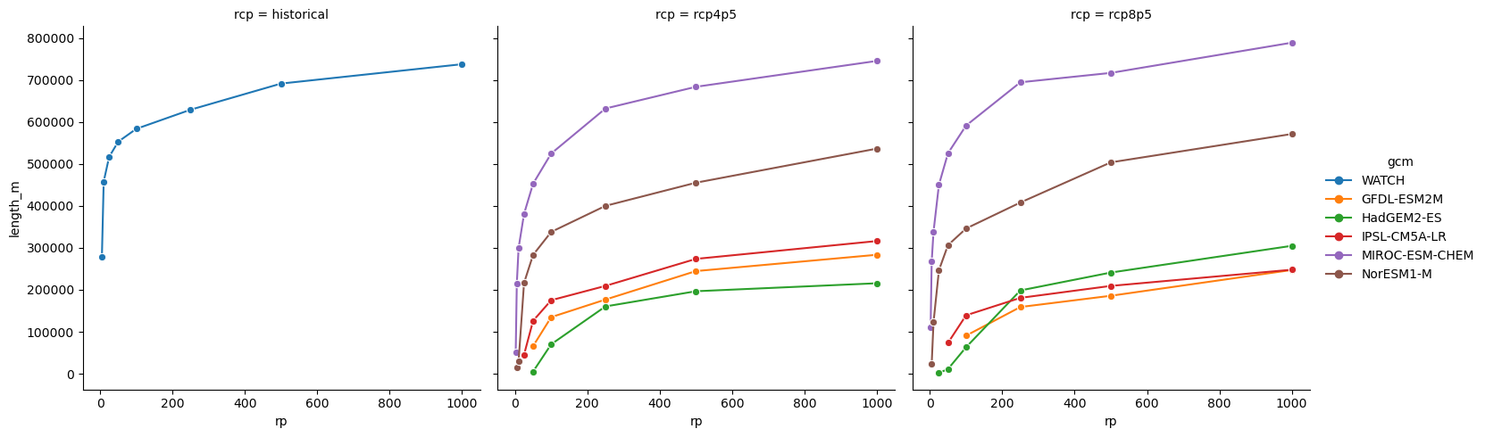
Summarise total length of roads exposed to depth 2m or greater river flooding, under different return periods and climate scenarios:
[15]:
summary = (
    river[river.depth_m >= 2.0]
    .drop(columns=["id", "split", "road_type", "key"])
    .groupby(["hazard", "rcp", "gcm", "epoch", "rp"])
    .sum()
    .drop(columns=["depth_m"])
)

summary
[15]:
| length_m | |||||
|---|---|---|---|---|---|
| hazard | rcp | gcm | epoch | rp | |
| inunriver | historical | WATCH | 1980 | 00005 | 278185.204955 |
| 00010 | 458024.929099 | ||||
| 00025 | 516672.545158 | ||||
| 00050 | 552825.932679 | ||||
| 00100 | 583449.265549 | ||||
| ... | ... | ... | ... | ... | |
| rcp8p5 | NorESM1-M | 2080 | 00050 | 306446.190164 | |
| 00100 | 346057.864928 | ||||
| 00250 | 407998.269230 | ||||
| 00500 | 503666.482039 | ||||
| 01000 | 571243.766343 |
208 rows × 1 columns
Plot exposure against return period, with separate plot areas for each Representative Concentration Pathway (RCP), and different colours for the different Global Climate Models (GCM):
[16]:
plot_data = summary.reset_index()
plot_data = plot_data[plot_data.epoch.isin(["1980", "2080"])]
plot_data.rp = plot_data.rp.apply(lambda rp: int(rp.lstrip("0")))
plot_data["probability"] = 1 / plot_data.rp
plot_data.head(5)
[16]:
| hazard | rcp | gcm | epoch | rp | length_m | probability | |
|---|---|---|---|---|---|---|---|
| 0 | inunriver | historical | WATCH | 1980 | 5 | 278185.204955 | 0.20 |
| 1 | inunriver | historical | WATCH | 1980 | 10 | 458024.929099 | 0.10 |
| 2 | inunriver | historical | WATCH | 1980 | 25 | 516672.545158 | 0.04 |
| 3 | inunriver | historical | WATCH | 1980 | 50 | 552825.932679 | 0.02 |
| 4 | inunriver | historical | WATCH | 1980 | 100 | 583449.265549 | 0.01 |
[17]:
sns.relplot(
    data=plot_data,
    x="rp",
    y="length_m",
    hue="gcm",
    col="rcp",
    kind="line",
    marker="o",
)
[17]:
<seaborn.axisgrid.FacetGrid at 0x75248850be00>
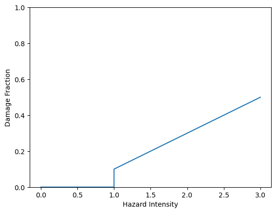
2. Vulnerability
Set up fragility curve assumptions, where probability of damage (pfail) depends on whether a road is paved and the depth of flood it is exposed to.
These assumptions are derived from Koks, E.E., Rozenberg, J., Zorn, C. et al. A global multi-hazard risk analysis of road and railway infrastructure assets. Nat Commun 10, 2677 (2019). https://doi.org/10.1038/s41467-019-10442-3, Figure S3, extrapolated to 2m and 3m depths.
The analysis is likely to be highly sensitive to these assumptions, and this approach is strongly limited by the availability and quality of fragility data, as well as the assumption that fragility can be related to flood depth alone - flood water velocity would be an important factor in a more detailed vulnerability assessment.
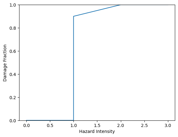
[18]:
paved = snail.damages.PiecewiseLinearDamageCurve(
    pd.DataFrame(
        {
            "intensity": [0.0, 0.999999999, 1, 2, 3],
            "damage": [0.0, 0.0, 0.1, 0.3, 0.5],
        }
    )
)
unpaved = snail.damages.PiecewiseLinearDamageCurve(
    pd.DataFrame(
        {
            "intensity": [0.0, 0.999999999, 1, 2, 3],
            "damage": [0.0, 0.0, 0.9, 1.0, 1.0],
        }
    )
)
paved, unpaved
[18]:
(<snail.damages.PiecewiseLinearDamageCurve at 0x75242c8b16a0>,
 <snail.damages.PiecewiseLinearDamageCurve at 0x75242c921590>)
[19]:
paved.plot(), unpaved.plot()
[19]:
(<Axes: xlabel='Hazard Intensity', ylabel='Damage Fraction'>,
 <Axes: xlabel='Hazard Intensity', ylabel='Damage Fraction'>)
Set up cost assumptions.
These are taken from Koks et al (2019) again, Table S8, construction costs to be assumed as an estimate of full rehabilitation after flood damage.
Again the analysis is likely to be highly sensitive to these assumptions, which should be replaced by better estimates if available.
[20]:
costs = pd.DataFrame(
    {
        "kind": ["paved_four_lane", "paved_two_lane", "unpaved"],
        "cost_usd_per_km": [3_800_000, 932_740, 22_780],
    }
)
costs
[20]:
| kind | cost_usd_per_km | |
|---|---|---|
| 0 | paved_four_lane | 3800000 |
| 1 | paved_two_lane | 932740 |
| 2 | unpaved | 22780 |
Set up assumptions about which roads are paved or unpaved, and number of lanes.
[21]:
sorted(river.road_type.unique())
[21]:
['motorway',
 'motorway_link',
 'primary',
 'primary_link',
 'secondary',
 'secondary_link',
 'tertiary',
 'tertiary_link',
 'trunk',
 'trunk_link']
Assume all tertiary roads are unpaved, all others are paved.
[22]:
river["paved"] = ~(river.road_type == "tertiary")
[23]:
def kind(road_type):
    if road_type in ("trunk", "trunk_link", "motorway"):
        return "paved_four_lane"
    elif road_type in ("primary", "primary_link", "secondary"):
        return "paved_two_lane"
    else:
        return "unpaved"


river["kind"] = river.road_type.apply(kind)
[24]:
river = river.merge(costs, on="kind")
Use the damage curve to estimate proportion_damaged for each exposed section.
[25]:
river.head(2)
[25]:
| id | split | road_type | length_m | key | depth_m | hazard | rcp | gcm | epoch | rp | paved | kind | cost_usd_per_km | |
|---|---|---|---|---|---|---|---|---|---|---|---|---|---|---|
| 0 | roade_55 | 0 | trunk | 256.660267 | wri_aqueduct-version_2-inunriver_historical_00... | 2.243539 | inunriver | historical | WATCH | 1980 | 00005 | True | paved_four_lane | 3800000 |
| 1 | roade_126 | 0 | trunk | 364.644366 | wri_aqueduct-version_2-inunriver_historical_00... | 0.073757 | inunriver | historical | WATCH | 1980 | 00005 | True | paved_four_lane | 3800000 |
[26]:
paved_depths = river.loc[river.paved, "depth_m"]
paved_damage = paved.damage_fraction(paved_depths)
river.loc[river.paved, "proportion_damaged"] = paved_damage

unpaved_depths = river.loc[~river.paved, "depth_m"]
unpaved_damage = paved.damage_fraction(unpaved_depths)
river.loc[~river.paved, "proportion_damaged"] = unpaved_damage
Finally estimate cost of rehabilitation for each exposed section
[27]:
river["damage_usd"] = river.length_m * river.cost_usd_per_km * 1e-3
river.head(2)
[27]:
| id | split | road_type | length_m | key | depth_m | hazard | rcp | gcm | epoch | rp | paved | kind | cost_usd_per_km | proportion_damaged | damage_usd | |
|---|---|---|---|---|---|---|---|---|---|---|---|---|---|---|---|---|
| 0 | roade_55 | 0 | trunk | 256.660267 | wri_aqueduct-version_2-inunriver_historical_00... | 2.243539 | inunriver | historical | WATCH | 1980 | 00005 | True | paved_four_lane | 3800000 | 0.348708 | 9.753090e+05 |
| 1 | roade_126 | 0 | trunk | 364.644366 | wri_aqueduct-version_2-inunriver_historical_00... | 0.073757 | inunriver | historical | WATCH | 1980 | 00005 | True | paved_four_lane | 3800000 | 0.000000 | 1.385649e+06 |
[28]:
river.to_csv(data_folder / "results" / "inunriver_damages_rp.csv", index=False)
[29]:
summary = (
    river.drop(
        columns=[
            "id",
            "split",
            "length_m",
            "key",
            "depth_m",
            "paved",
            "kind",
            "cost_usd_per_km",
            "proportion_damaged",
        ]
    )
    .groupby(["road_type", "hazard", "rcp", "gcm", "epoch", "rp"])
    .sum()
)
summary
[29]:
| damage_usd | ||||||
|---|---|---|---|---|---|---|
| road_type | hazard | rcp | gcm | epoch | rp | |
| motorway | inunriver | historical | WATCH | 1980 | 00005 | 2.848222e+07 |
| 00010 | 2.848222e+07 | |||||
| 00025 | 2.848222e+07 | |||||
| 00050 | 2.848222e+07 | |||||
| 00100 | 2.848222e+07 | |||||
| ... | ... | ... | ... | ... | ... | ... |
| trunk_link | inunriver | rcp8p5 | NorESM1-M | 2080 | 00050 | 1.512558e+07 |
| 00100 | 1.512558e+07 | |||||
| 00250 | 1.512558e+07 | |||||
| 00500 | 1.512558e+07 | |||||
| 01000 | 1.512558e+07 |
2780 rows × 1 columns
3. Risk
Calculate expected annual damages for each road under historical hazard.
Start by selecting only historical intersections, and keeping only the road ID, return period, and cost of rehabilitation if damaged.
[30]:
historical = river[river.rcp == "historical"][["id", "rp", "damage_usd"]]
Sum up the expected damage for each road, per return period, then pivot the table to create columns for each return period - now there is one row per road.
[31]:
historical = historical.groupby(["id", "rp"]).sum().reset_index()
historical = historical.pivot(index="id", columns="rp").replace(float("NaN"), 0)
historical.columns = [f"rp{int(rp)}" for _, rp in historical.columns]
historical.head(2)
[31]:
| rp5 | rp10 | rp25 | rp50 | rp100 | rp250 | rp500 | rp1000 | |
|---|---|---|---|---|---|---|---|---|
| id | ||||||||
| roade_10001 | 386658.527135 | 386658.527135 | 386658.527135 | 386658.527135 | 386658.527135 | 386658.527135 | 386658.527135 | 386658.527135 |
| roade_10002 | 11485.501119 | 11485.501119 | 11485.501119 | 11485.501119 | 11485.501119 | 11485.501119 | 11485.501119 | 11485.501119 |
Calculate expected annual damages, integrating under the expected damage curve over return periods.
[32]:
def calculate_ead(df):
    rp_cols = sorted(list(df.columns), key=lambda col: 1 / int(col.replace("rp", "")))
    rps = np.array([int(col.replace("rp", "")) for col in rp_cols])
    probabilities = 1 / rps
    rp_damages = df[rp_cols]
    return simpson(rp_damages, x=probabilities, axis=1)


historical["ead_usd"] = calculate_ead(historical)
historical.head(2)
[32]:
| rp5 | rp10 | rp25 | rp50 | rp100 | rp250 | rp500 | rp1000 | ead_usd | |
|---|---|---|---|---|---|---|---|---|---|
| id | |||||||||
| roade_10001 | 386658.527135 | 386658.527135 | 386658.527135 | 386658.527135 | 386658.527135 | 386658.527135 | 386658.527135 | 386658.527135 | 76945.046900 |
| roade_10002 | 11485.501119 | 11485.501119 | 11485.501119 | 11485.501119 | 11485.501119 | 11485.501119 | 11485.501119 | 11485.501119 | 2285.614723 |
[33]:
historical.to_csv(data_folder / "results" / "inunriver_damages_ead__historical.csv")
4. Future risk
Calculate expected annual damages under each future scenario (for each global climate model and representative concentration pathway).
This follows the same method as for historical flooding above, with the added variables of climate model and rcp.
[34]:
future = river[["id", "rp", "rcp", "gcm", "epoch", "damage_usd"]].copy()
Sum up the expected damage for each road, per return period, gcm and rcp
[35]:
future = future.groupby(["id", "rp", "rcp", "gcm", "epoch"]).sum().reset_index()
future.head(2)
[35]:
| id | rp | rcp | gcm | epoch | damage_usd | |
|---|---|---|---|---|---|---|
| 0 | roade_10001 | 00002 | rcp4p5 | GFDL-ESM2M | 2030 | 386658.527135 |
| 1 | roade_10001 | 00002 | rcp4p5 | GFDL-ESM2M | 2050 | 386658.527135 |
Pivot the table to create columns for each return period - now there is one row per road, gcm and rcp.
[36]:
future = future.pivot(index=["id", "rcp", "gcm", "epoch"], columns="rp").replace(
    float("NaN"), 0
)
future.columns = [f"rp{int(rp)}" for _, rp in future.columns]
future.head(2)
[36]:
| rp2 | rp5 | rp10 | rp25 | rp50 | rp100 | rp250 | rp500 | rp1000 | ||||
|---|---|---|---|---|---|---|---|---|---|---|---|---|
| id | rcp | gcm | epoch | |||||||||
| roade_10001 | historical | WATCH | 1980 | 0.000000 | 386658.527135 | 386658.527135 | 386658.527135 | 386658.527135 | 386658.527135 | 386658.527135 | 386658.527135 | 386658.527135 |
| rcp4p5 | GFDL-ESM2M | 2030 | 386658.527135 | 386658.527135 | 386658.527135 | 386658.527135 | 386658.527135 | 386658.527135 | 386658.527135 | 386658.527135 | 386658.527135 |
Calculate expected annual damages, integrating under the expected damage curve over return periods.
[37]:
future["ead_usd"] = calculate_ead(future)
[38]:
future.to_csv(data_folder / "results" / "inunriver_damages_ead.csv")
Pick out an individual road by id, to spot check uncertainty:
[39]:
future.reset_index().id.unique()
[39]:
array(['roade_10001', 'roade_10002', 'roade_10011', ..., 'roade_9925',
       'roade_9926', 'roade_9930'], shape=(2363,), dtype=object)
[40]:
# future.loc["roade_1002"]
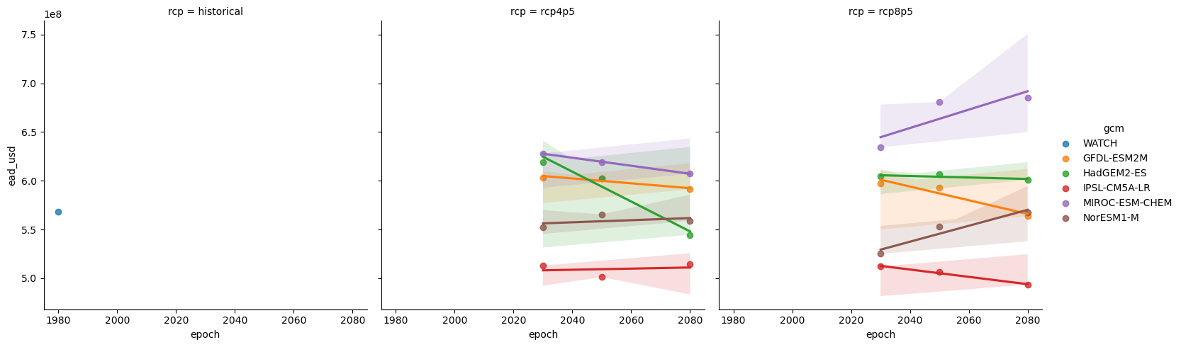
Summarise total expected annual (direct) damages, showing variation between climate models and representative concentration pathways.
[41]:
summary = (
    future.reset_index()[["rcp", "gcm", "epoch", "ead_usd"]]
    .groupby(["rcp", "gcm", "epoch"])
    .sum()
    .reset_index()
)
summary.epoch = summary.epoch.astype(int)
summary.head()
[41]:
| rcp | gcm | epoch | ead_usd | |
|---|---|---|---|---|
| 0 | historical | WATCH | 1980 | 5.679075e+08 |
| 1 | rcp4p5 | GFDL-ESM2M | 2030 | 6.031936e+08 |
| 2 | rcp4p5 | GFDL-ESM2M | 2050 | 6.025140e+08 |
| 3 | rcp4p5 | GFDL-ESM2M | 2080 | 5.912566e+08 |
| 4 | rcp4p5 | HadGEM2-ES | 2030 | 6.193782e+08 |
[42]:
sns.lmplot(
    data=summary,
    col="rcp",
    x="epoch",
    y="ead_usd",
    hue="gcm",  # fit_reg=False
)
[42]:
<seaborn.axisgrid.FacetGrid at 0x75242c7e60d0>